Workshops

iMADE Workshops
Current location: Home > Workshops > iMADE Workshops

Workshop #5 Supervised Learning: FFBPN

Posted:2021-04-19 08:43:57　Click:1488

An introduction to backpropagation

Neural networks, like any other supervised learning algorithms, learn to map an input to an output based on some provided examples of (input, output) pairs, called the training set. In particular, neural networks performs this mapping by processing the input through a set of transformations. A neural network is composed of several layers, and each of these layers are made of units (also called neurons) as illustrated below:

In the picture above, the input is transformed first through the hidden layer 1, then the second one and finally an output is predicted. Each transformation is controlled by a set of weights (and biases). During training, to indeed learn something, the network needs to adjust these weights to minimize the error (also called the loss function) between the expected outputs and the ones it maps from the given inputs. Using gradient descent as an optimization algorithm, the weights are updated at each iteration as:

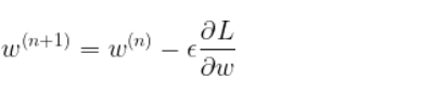
where L is the loss function and $\large \epsilon$ is the learning rate.

As we can see above, the gradient of the loss with respect to the weight is substracted from the weight at each iteration. This is the so called gradient descent. The gradient $\large \dpi{100} \large \frac{\partial L}{\partial w}$ can be interpreted as a measure of the contribution of the weight to the loss. Therefore the larger is this gradient (in absolute value), the more the weight is updated during an iteration of gradient descent.

The minimization of the loss function task ends up being related to the evaluation of the gradients described above. We will review 3 proposals to perform this evaluation:

Analytical calculation of the gradients.
Approximation of the gradients as being: $\large \dpi{100} \large \frac{\partial L}{\partial w} = \frac{L(w + \delta w) - L(w)}{\delta w}$ , where $\large \dpi{100} \large \delta w \rightarrow 0$ .
Backpropagation or reverse mode autodiff.

Before going into the details of these proposals, we will first clearly define our problem and simplify it for the sake of the discussion.

Problem Definition

Let's discuss a little bit about how the input is transformed to produce the hidden layer representation. In neural network, a layer is obtained by performing two operations on the previous layer:

First the previous layer is tranformed via a linear operation: the value of the previous layer is multiplied by a weight, and a bias is added to it. It gives: $\large z= xw + b$ , where $\large x$ is the value of the previous layer unit, $\large w$ and $\large b$ are respectively the weight and the bias discussed above.
Second, the previous linear operation is used as an input to the activation function of the unit. This activation is generally chosen to introduce non linearity in order to solve complex tasks. Here we will simply consider that this activation function is a sigmoid function: $\large \sigma(x) = \frac{1}{1+\exp(-x)}$ . As a consequence the value y of a layer can be written as: $\large y = \sigma (z) = \sigma (xw + b)$ .

So now, considering our case, with an input layer, one hidden layer, and an output layer, all made of a single unit and respectively called x, h and y, we can write:

$\large h = \sigma (xw_1 + b_1)$ , where $\large w_1$ and $\large b_1$ are respectively the weight and the bias used to compute the hidden unit from the input.

$\large y = \sigma (hw_2 + b_2)$ , where $\large w_2$ and $\large b_2$ are respectively the weight and the bias used to compute the output from the hidden unit.

From now on, we are able to calculate the output y based on the input x, through a set of transformations. This is the so called forward propagation since this calculation goes forward inside the network.

We now need to compare this predicted ouptut to the true one $\large y_T$ . As explained earlier, we use a loss function to quantify the error that the network does while prediciting. Here we will consider as a loss function the squared error defined as :

$\large L = \frac{1}{2} (y-y_T)^2$

As discussed earlier, the weights (and biases) need to be updated according to the gradient of this loss function L with respect to these weights (and biases). Therefore the challenge here is to evaluate these gradients. The first approach would be to manually derive them.

Analytical differentiation

Although this method is cumbersome and error prone, it is worth to investigate to better understand the challenge Here we simplify a lot the problem since we have a single hidden layer and a single unit per layer. And yet the analytical derivation requires quite some attention.

$\large \frac{\partial L}{\partial w_2} = \frac{1}{2} \frac{\partial \left((y-y_T)^2\right)}{\partial w_2}=\frac{1}{2} \left(\frac{\partial \left(y^2\right)}{\partial w_2} - 2y_T \frac{\partial y}{\partial w_2}\right)$

Knowing that $\large y = \sigma (hw_2 +b_2)$ , we get :

$\large \frac{\partial L}{\partial w_2} = \frac{1}{2} \left(\frac{\partial \left(\frac{1}{\left( 1 + \exp(-hw_2 -b_2\right))^2}\right)}{\partial w_2} - 2y_T \frac{\partial \frac{1}{1 + \exp(-hw_2 - b_2)}}{\partial w_2}\right)=h\frac{ \exp(-hw_2 - b_2)}{\left(1+\exp(-hw_2 - b_2)\right)^2} \left(\frac{1}{1+\exp(-hw_2 - b_2)} - y_T\right)$

Here we derived the gradient with respect to $w_2$ , and the calculation for the one with respect with $\large w_1$ would be even more tedious. Therefore such an analytical approach would be very hard to implement for a complex network. In addition, computing wise this approach would be quite inefficient since we could not leverage the fact that the gradients share some common definition as we will soon discuss. A way more easy way to get these gradients would be to use a numerical approximation.

Numerical differentiation

Trading accuracy for simplicity, we can obtain the gradient using the following :

$\large \frac{\partial L}{\partial w} \simeq \frac{L(w + \delta w) - L(w)}{\delta w}$ , with $\large \delta w \rightarrow 0$

As suggested above, although simpler than the analytical derivation, this numerical differentiation is also less precise. In addition for every gradients to evaluate, we would have to calculate the loss function at least once (doing one forward pass by weights and biases). For a neural network with 1 million weigth parameters, it would requires 1 million forward passes, which is definitely not efficient to compute. Let's now come to a better solution and the core of this article by reviewing the backpropagation approach.

Backpropagation

Before speaking in more details about what backpropagation is, let's first introduce the computational graph that leads to the evaluation of the loss function.

The nodes in this graph correspond to all the values that are computed in order to get the loss L. If a variable is computed by applying an operation to another variable, an edge is drawn between the two variable nodes. Looking at this graph, and making use of the chain rule of calculus, we can express the gradient of L with respect to the weights (or biases) as:

$\large \frac{\partial L}{\partial w_2} = \frac{\partial L}{\partial y} \frac{\partial y}{\partial w_2} = \frac{\partial L}{\partial y} \frac{\partial y}{\partial z_2}\frac{\partial z_2}{\partial w_2}$

Same goes for the weight $\large w_1$ :

$\large \frac{\partial L}{\partial w_1} = \frac{\partial L}{\partial y} \frac{\partial y}{\partial w_1} = \frac{\partial L}{\partial y} \frac{\partial y}{\partial z_2} \frac{\partial z_2}{\partial w_1} = \frac{\partial L}{\partial y} \frac{\partial y}{\partial z_2} \frac{\partial z_2}{\partial h} \frac{\partial h}{\partial w_1} = \frac{\partial L}{\partial y} \frac{\partial y}{\partial z_2} \frac{\partial z_2}{\partial h} \frac{\partial h}{\partial z_1} \frac{\partial z_1}{\partial w_1}$

One very important thing to notice here is that the evaluation of the gradient $\large \frac{\partial L}{\partial w_1}$ can reuse some of the calculations perfomed during the evaluation of the gradient $\large \frac{\partial L}{\partial w_2}$ . It is even clearer if we evaluate the gradient $\large \frac{\partial L}{\partial b_1}$ :

$\large \frac{\partial L}{\partial b_1} = \frac{\partial L}{\partial y} \frac{\partial y}{\partial z_2} \frac{\partial z_2}{\partial h} \frac{\partial h}{\partial z_1} \frac{\partial z_1}{\partial b_1}$

We see that the first four terms on the righ hand of the equation are the same than the one from $\large \frac{\partial L}{\partial w_1}$ .

As you can see in the equations above, we calculate the gradient starting from the end of the computational graph, and proceed backward to get the gradient of the loss with respect to the weights (or the biases). This backward evaluation gives its name to the algoritm: backpropagation. The backpropagation algorithm can be illustrated by the image below:

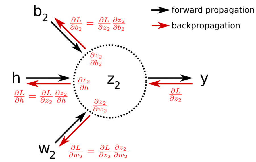
In pratice, one iteration of gradient descent would now require one forward pass, and only one pass in the reverse direction computing all the partial derivatives starting from the output node. It is therefore way more efficient than the previous approaches. In the original paper about backpropagation published in 1986 , the authors (among which Geoffrey Hinton) used for the first time backpropagation to allow internal hidden units to learn features of the task domain.

Backpropagation Algorithm

Backpropagation Parameters

Refer to the website：https://keras.io/api/

Backpropagation task

Use BP Neural Network to Predict Financial Trends

/Public/Uploadfiles/20210421/20210421023714_32456.zip