Introduction

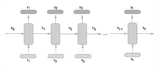
Recurrent neural networks is a type of deep learning-oriented algorithm, which follows a sequential approach. In neural networks, we always assume that each input and output is independent of all other layers. These type of neural networks are called recurrent because they perform mathematical computations in sequential manner.

Consider the following steps to train a recurrent neural network −

Step 1 − Input a specific example from dataset.

Step 2 − Network will take an example and compute some calculations using randomly initialized variables.

Step 3 − A predicted result is then computed.

Step 4 − The comparison of actual result generated with the expected value will produce an error.

Step 5 − To trace the error, it is propagated through same path where the variables are also adjusted.

Step 6 − The steps from 1 to 5 are repeated until we are confident that the variables declared to get the output are defined properly.

Step 7 − A systematic prediction is made by applying these variables to get new unseen input.

The schematic approach of representing recurrent neural networks is described below −

Recurrent Neural Network Implementation with TensorFlow

In this section, we will learn how to implement recurrent neural network with TensorFlow.

In this section, we will learn how to implement recurrent neural network with TensorFlow.

Step 1 − TensorFlow includes various libraries for specific implementation of the recurrent neural network module.

# Import Library Packages import tensorflow as tf from tensorflow.contrib import rnn import numpy as np import matplotlib.pyplot as plt import time

Step 2 − Our primary motive is to classify the images using a recurrent neural network, where we consider every image row as a sequence of pixels. MNIST image shape is specifically defined as 28*28 px. Now we will handle 28 sequences of 28 steps for each sample that is mentioned. We will define the input parameters to get the sequential pattern done.

# Import MNIST data from tensorflow.examples.tutorials.mnist import input_data mnist = input_data.read_data_sets("/tmp/data/", one_hot=True)

Step 3 − Define all the RNN related parameters and settings

# Training Parameters learning_rate = 0.001 training_steps = 10000 batch_size = 128 display_step = 200 # Network Parameters num_input = 28 # MNIST data input (img shape: 28*28) timesteps = 28 # timesteps num_hidden = 128 # hidden layer num of features num_classes = 10 # MNIST total classes (0-9 digits)

Step 4 − Define X & Y placeholders

# tf Graph input X = tf.placeholder("float", [None, timesteps, num_input]) Y = tf.placeholder("float", [None, num_classes])

Step 5 − Define network weights and biases

# Define weights weights = { 'out': tf.Variable(tf.random_normal([num_hidden, num_classes])) } biases = { 'out': tf.Variable(tf.random_normal([num_classes])) }

Step 6 − Define plot settings

#Plot settings avg_set = [] epoch_set = []

Step 7 − Define the RNN,  loss and optimizer and all variable initialization.

def RNN(x, weights, biases): # Prepare data shape to match `rnn` function requirements # Current data input shape: (batch_size, timesteps, n_input) # Required shape: 'timesteps' tensors list of shape (batch_size, n_input) # Unstack to get a list of 'timesteps' tensors of shape (batch_size, n_input) x = tf.unstack(x, timesteps, 1) # Define a lstm cell with tensorflow lstm_cell = rnn.BasicLSTMCell(num_hidden, forget_bias=1.0) # Get lstm cell output outputs, states = rnn.static_rnn(lstm_cell, x, dtype=tf.float32) # Linear activation, using rnn inner loop last output return tf.matmul(outputs[-1], weights['out']) + biases['out'] logits = RNN(X, weights, biases) prediction = tf.nn.softmax(logits) # Define loss and optimizer loss_op = tf.reduce_mean(tf.nn.softmax_cross_entropy_with_logits( logits=logits, labels=Y)) optimizer = tf.train.GradientDescentOptimizer(learning_rate=learning_rate) train_op = optimizer.minimize(loss_op) # Evaluate model (with test logits, for dropout to be disabled) correct_pred = tf.equal(tf.argmax(prediction, 1), tf.argmax(Y, 1)) accuracy = tf.reduce_mean(tf.cast(correct_pred, tf.float32)) # Initialize the variables (i.e. assign their default value) init = tf.global_variables_initializer()

Step 8 − Execute the RNN training session

# Start training with tf.Session() as sess: # Run the initializer sess.run(init) for step in range(1, training_steps+1): batch_x, batch_y = mnist.train.next_batch(batch_size) # Reshape data to get 28 seq of 28 elements batch_x = batch_x.reshape((batch_size, timesteps, num_input)) # Run optimization op (backprop) sess.run(train_op, feed_dict={X: batch_x, Y: batch_y}) if step % display_step == 0 or step == 1: # Calculate batch loss and accuracy loss, acc = sess.run([loss_op, accuracy], feed_dict={X: batch_x, Y: batch_y}) print("Step " + str(step) + ", Minibatch Loss= " + \ "{:.4f}".format(loss) + ", Training Accuracy= " + \ "{:.3f}".format(acc)) avg_set.append(acc) epoch_set.append(step + 1) print("Optimization Finished!") # Calculate accuracy for 128 mnist test images test_len = 128 test_data = mnist.test.images[:test_len].reshape((-1, timesteps, num_input)) test_label = mnist.test.labels[:test_len] print("Testing Accuracy:", \ sess.run(accuracy, feed_dict={X: test_data, Y: test_label}))

Step 9 − Plot the RNN performance chart

plt.plot(epoch_set, avg_set, 'o', label = 'RNN Training phase') plt.ylabel('accuracy') plt.xlabel('epoch') plt.legend() plt.show()

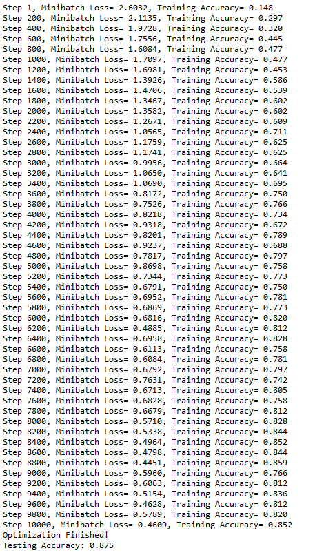
The screenshots below show the output generated −

The RNN Performance Chart should look like this: