AutoEncoders

An AE is a network with three or more layers, where the input layer and the output have the same number of neurons, and those intermediate (hidden layers) have a lower number of neurons.

The network is trained to simply reproduce in the output, for each piece of input data, the same pattern of activity in the input.

AEs are ANNs capable of learning efficient representations of the input data without any supervision (that is, the training set is unlabeled).

They typically have a much lower dimensionality than the input data, making AEs useful for dimensionality reduction.

More importantly, AEs act as powerful feature detectors, and they can be used for unsupervised pre-training of DNNs.

The remarkable aspect of the problem is that, due to the lower number of neurons in the hidden layer, if the network can learn from examples and generalize to an acceptable extent, it performs data compression; the status of the hidden neurons provides, for each example, a compressed version of the input and output common states.

Useful applications of AEs are data denoising and dimensionality reduction for data visualization.

The following diagram shows how an AE typically works; it reconstructs the received input through two phases: an encoding phase, which corresponds to a dimensional reduction for the original input, and a decoding phase, which is capable of reconstructing the original input from the encoded (compressed) representation

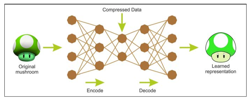
Fig. 1 Encoder and decoder phases in an autoencoder

As an unsupervised neural network, the main characteristic of an autoencoder is its symmetrical structure.

An autoencoder has two components: an encoder that converts the input to an internal representation, followed by a decoder that converts the internal representation to the output.

In other words, an autoencoder can be seen as a combination of an encoder, where we encode some input into a code, and a decoder, where we decode/reconstruct the code back to its original input as the output.

Thus, an MLP typically has the same architecture as an autoencoder, except that the number of neurons in the output layer must be equal to the number of inputs.

As mentioned previously, there is more than one way to train an autoencoder.

The first way is to train the whole layer at once, similar to MLP.

However, instead of using some labeled output when calculating the cost function, as in supervised learning, we use the input itself.

Therefore, the cost function shows the difference between the actual input and the reconstructed input.

The following diagram shows an autoencoder that consists of the narrow hidden layer between an encoder and a decoder:

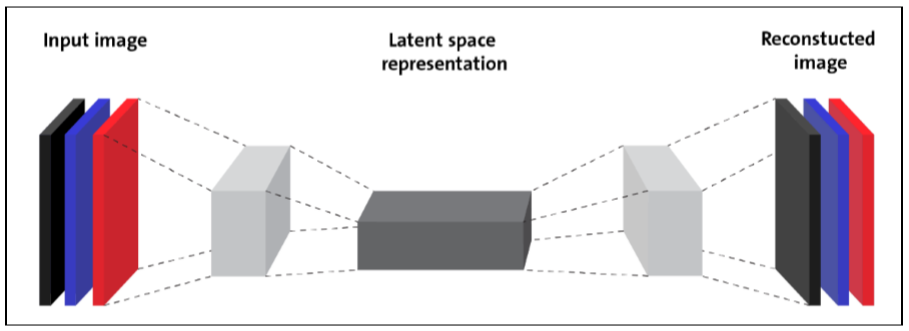
Fig. 2 An unsupervised autoencoder as a network for latent feature learning

The system architecture of autoencoder is shown in Fig. 3.

Fig. 3 Learning an approximation of the identity function autoencoder

As a concrete example, suppose the inputs x are the pixel intensity values of a 10 × 10 image (100 pixels), so n=100, and there are 50 = hidden units in layer L2.

Since there are only 50 hidden units, the network is forced to learn a compressed representation of the input.

It is only given the vector of hidden unit activations, so it must try to reconstruct the 100-pixel input, that is, x1, x2, …, x100 from the 50 hidden units.

The preceding diagram shows only 6 inputs feeding into layer 1 and exactly 6 units feeding out from layer 3.

A neuron can be active (or firing) if its output value is close to 1, or inactive if its output value is close to 0.

However, for simplicity, we assume that the neurons are inactive most of the time.

This argument is true as long as we are talking about the sigmoid activation function.

However, if you are using the tanh function as an activation function, then a neuron is inactive when it outputs values close to -1.

Implementing autoencoders with TensorFlow

Dataset

In this article, we will be using MNIST, a data-set of handwritten digits (The “hello world” of image recognition for machine learning and deep learning).

Fig. 4 MNIST dataset

It is a digit recognition task. There are 10 digits (0 to 9) or 10 classes to predict. Each image is a 28 by 28 pixel square (784 pixels total). We’re given a total of 70,000 images.

Spyder

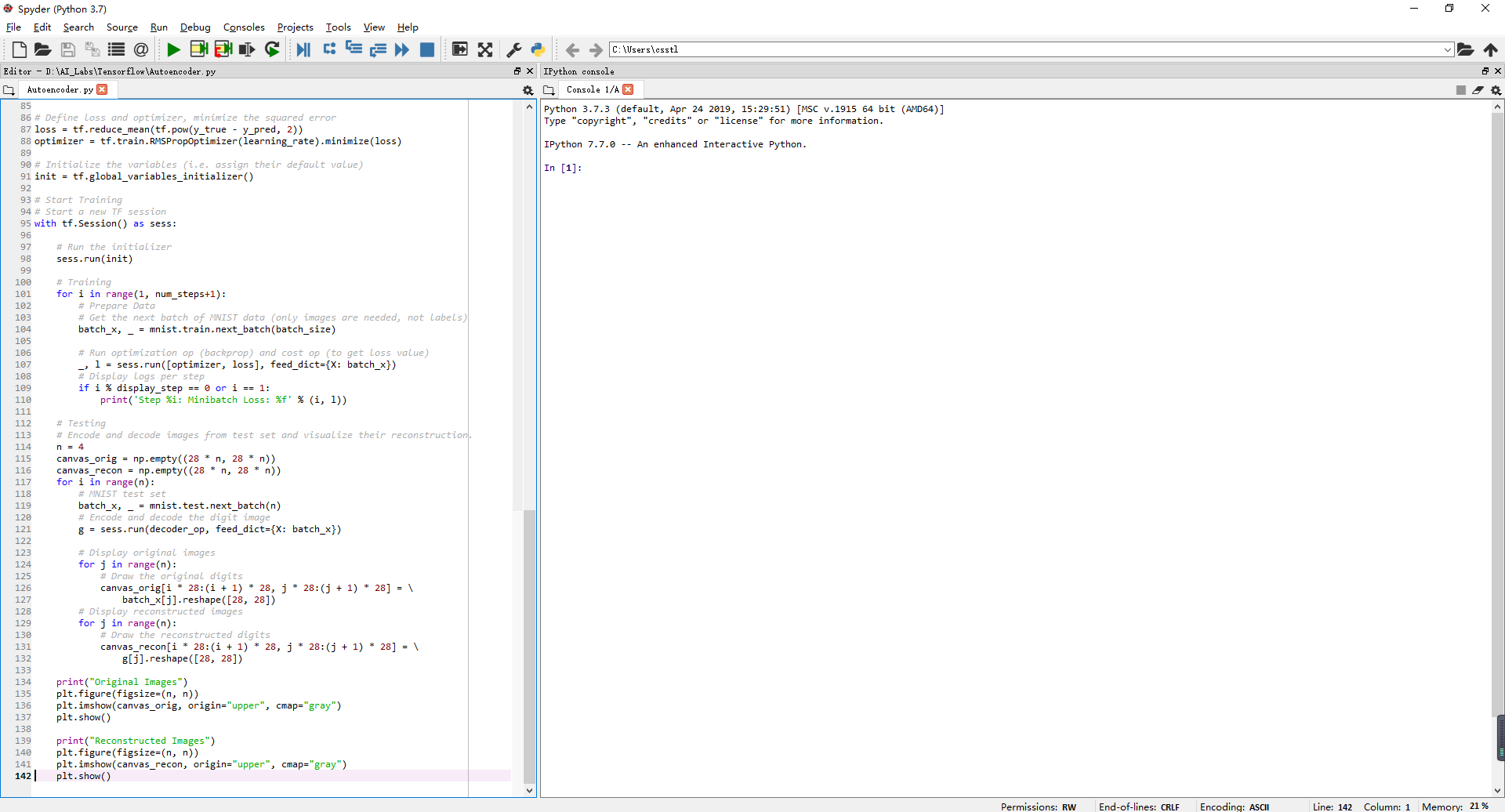
Launch the Spyder application by pressing the "Launch" button or run the Spyder application directly from the Windows menu. Like this.

Step 1 - Define the variables and treeNode class

# Import packages import tensorflow as tf import numpy as np import matplotlib.pyplot as plt

Step 2 - Import MNIST Data

# Import MNIST data from tensorflow.examples.tutorials.mnist import input_data mnist = input_data.read_data_sets("/tmp/data/", one_hot=True)

Step 3 - Define Training Parameters

# Training Parameters learning_rate = 0.01 num_steps = 30000 batch_size = 256 display_step = 1000 examples_to_show = 10

Step 4 - Define Network Parameters

# Network Parameters num_hidden_1 = 256 # 1st layer num features num_hidden_2 = 128 # 2nd layer num features (the latent dim) num_input = 784 # MNIST data input (img shape: 28*28)

Step 5 - Define tf Graph Input X

# tf Graph input (only pictures) X = tf.placeholder("float", [None, num_input])

Step 6 - Define weights and biases

weights = {     'encoder_h1': tf.Variable(tf.random_normal([num_input, num_hidden_1])),     'encoder_h2': tf.Variable(tf.random_normal([num_hidden_1, num_hidden_2])),     'decoder_h1': tf.Variable(tf.random_normal([num_hidden_2, num_hidden_1])),     'decoder_h2': tf.Variable(tf.random_normal([num_hidden_1, num_input])), } biases = {     'encoder_b1': tf.Variable(tf.random_normal([num_hidden_1])),     'encoder_b2': tf.Variable(tf.random_normal([num_hidden_2])),     'decoder_b1': tf.Variable(tf.random_normal([num_hidden_1])),     'decoder_b2': tf.Variable(tf.random_normal([num_input])), }

Step 7 - Define Plot Setting of Performance Chart

#Plot settings avg_set = [] epoch_set = []

Step 8 - Define encoder

# Building the encoder def encoder(x):     # Encoder Hidden layer with sigmoid activation #1     layer_1 = tf.nn.sigmoid(tf.add(tf.matmul(x, weights['encoder_h1']),                                    biases['encoder_b1']))     # Encoder Hidden layer with sigmoid activation #2     layer_2 = tf.nn.sigmoid(tf.add(tf.matmul(layer_1, weights['encoder_h2']),                                    biases['encoder_b2']))     return layer_2

Step 9 - Define decoder

# Building the decoder def decoder(x):     # Decoder Hidden layer with sigmoid activation #1     layer_1 = tf.nn.sigmoid(tf.add(tf.matmul(x, weights['decoder_h1']),                                    biases['decoder_b1']))     # Decoder Hidden layer with sigmoid activation #2     layer_2 = tf.nn.sigmoid(tf.add(tf.matmul(layer_1, weights['decoder_h2']),                                    biases['decoder_b2']))     return layer_2

Step 10 - Construct Autoencoder Model

# Construct model encoder_op = encoder(X) decoder_op = decoder(encoder_op)

Step 11 - Define Prediction Variable

# Prediction y_pred = decoder_op # Targets (Labels) are the input data. y_true = X

Step 12 - Define Loss and Optimizer

# Define loss and optimizer, minimize the squared error loss = tf.reduce_mean(tf.pow(y_true - y_pred, 2)) optimizer = tf.train.RMSPropOptimizer(learning_rate).minimize(loss)

Step 13 - Initialize All Variables

# Initialize the variables (i.e. assign their default value) init = tf.global_variables_initializer()

Step 14 - Start Training, display the  original images and decoded images

# Start Training # Start a new TF session with tf.Session() as sess:     # Run the initializer     sess.run(init)     # Training     for i in range(1, num_steps+1):         # Prepare Data         # Get the next batch of MNIST data (only images are needed, not labels)         batch_x, _ = mnist.train.next_batch(batch_size)         # Run optimization op (backprop) and cost op (to get loss value)         _, l = sess.run([optimizer, loss], feed_dict={X: batch_x})         # 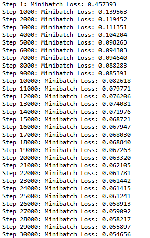Display logs per step         if i % display_step == 0 or i == 1:             print('Step %i: Minibatch Loss: %f' % (i, l))             avg_set.append(l)              epoch_set.append(i + 1)     # Testing     # Encode and decode images from test set and visualize their reconstruction.     n = 4     canvas_orig = np.empty((28 * n, 28 * n))     canvas_recon = np.empty((28 * n, 28 * n))     for i in range(n):         # MNIST test set         batch_x, _ = mnist.test.next_batch(n)         # Encode and decode the digit image         g = sess.run(decoder_op, feed_dict={X: batch_x})         # Display original images         for j in range(n):             # Draw the original digits             canvas_orig[i * 28:(i + 1) * 28, j * 28:(j + 1) * 28] = \                 batch_x[j].reshape([28, 28])         # Display reconstructed images         for j in range(n):             # Draw the reconstructed digits             canvas_recon[i * 28:(i + 1) * 28, j * 28:(j + 1) * 28] = \                 g[j].reshape([28, 28])     print("Original Images")     plt.figure(figsize=(n, n))     plt.imshow(canvas_orig, origin="upper", cmap="gray")     plt.show()     print("Reconstructed Images")     plt.figure(figsize=(n, n))     plt.imshow(canvas_recon, origin="upper", cmap="gray")     plt.show()          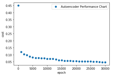plt.plot(epoch_set, avg_set, 'o', label = 'Autoencoder Performance Chart')      plt.ylabel('cost')      plt.xlabel('epoch')      plt.legend()      plt.show()

You should see the following results:

1. Training results

2. Output encoded and decoded images

3. System Performance Chart