Multilayer Preceptron - Introduction

Multi-Layer perceptron defines the most complicated architecture of artificial neural networks. It is substantially formed from multiple layers of perceptron.

The diagrammatic representation of multi-layer perceptron learning is as shown below −

Fig. 1 MLP System Architecture

MLP networks are usually used for supervised learning format. A typical learning algorithm for MLP networks is also called back propagation’s algorithm.

Now, we will focus on the implementation with MLP for an image classification problem.

TensorFlow

TensorFlow is an open source software library created by Google for numerical computation using data flow graphs.

Nodes in the graph represent mathematical operations, while the graph edges represent the multidimensional data arrays (tensors) that flow between them. This flexible architecture lets you deploy computation to one or more CPU's or GPU’s in a desktop, server, or mobile device without rewriting code.

TensorFlow also includes TensorBoard, a data visualization toolkit.

Building a MLP in TensorFlow

Dataset

In this article, we will be using MNIST, a data-set of handwritten digits (The “hello world” of image recognition for machine learning and deep learning).

Fig. 2 MNIST Sample Images

It is a digit recognition task. There are 10 digits (0 to 9) or 10 classes to predict. Each image is a 28 by 28 pixel square (784 pixels total). We’re given a total of 70,000 images.

Python Code

Step 1 - Launch Python TensorFlow (eg.) from Anaconda Spyder

Step 2 - Import Packages

import tensorflow as tf import numpy as np import matplotlib.pyplot as plt %matplotlib inline import time

Step 3 - Load MNIST Data

# Import MNIST data from tensorflow.examples.tutorials.mnist import input_data mnist = input_data.read_data_sets("/tmp/data/", one_hot=True)

You should see something like this:

Extracting data/MNIST/train-images-idx3-ubyte.gz
Extracting data/MNIST/train-labels-idx1-ubyte.gz
Extracting data/MNIST/t10k-images-idx3-ubyte.gz
Extracting data/MNIST/t10k-labels-idx1-ubyte.gz

Check the data by typing:

print("Size of:") print("- Training-set:\t\t{}".format(len(data.train.labels))) print("- Test-set:\t\t{}".format(len(data.test.labels))) print("- Validation-set:\t{}".format(len(data.validation.labels)))

You should see something like this:

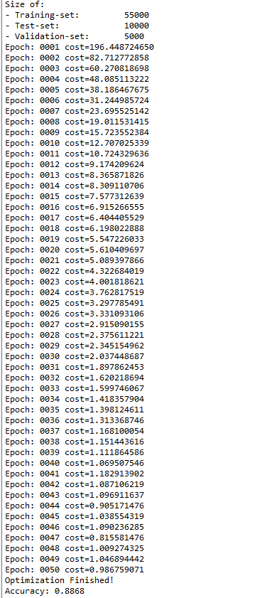
Size of:
- Training-set: 55000
- Test-set: 10000
- Validation-set: 5000

Step 4 - Set MLP Parameters

# Parameters learning_rate = 0.01 training_epochs = 50 batch_size = 100 display_step = 1

Step 5 - Set MLP Network Parameters

# Network Parameters n_hidden_1 = 256 # 1st layer number of neurons n_hidden_2 = 256 # 2nd layer number of neurons n_input = 784 # MNIST data input (img shape: 28*28) n_classes = 10 # MNIST total classes (0-9 digits)

Step 6 - Set X & Y Placeholders

# tf Graph input X = tf.placeholder("float", [None, n_input]) Y = tf.placeholder("float", [None, n_classes])

Step 7 - Define weights and bias

# Store layers weight & bias weights = { 'h1': tf.Variable(tf.random_normal([n_input, n_hidden_1])), 'h2': tf.Variable(tf.random_normal([n_hidden_1, n_hidden_2])), 'out': tf.Variable(tf.random_normal([n_hidden_2, n_classes])) } biases = { 'b1': tf.Variable(tf.random_normal([n_hidden_1])), 'b2': tf.Variable(tf.random_normal([n_hidden_2])), 'out': tf.Variable(tf.random_normal([n_classes])) }

Step 8 - Define plot settings (Average cost vs. Epochs)

# Plot settings avg_set = [] epoch_set = []

Step 9 - Create MLP Model

# Create model def multilayer_perceptron(x): # Hidden fully connected layer with 256 neurons layer_1 = tf.add(tf.matmul(x, weights['h1']), biases['b1']) # Hidden fully connected layer with 256 neurons layer_2 = tf.add(tf.matmul(layer_1, weights['h2']), biases['b2']) # Output fully connected layer with a neuron for each class out_layer = tf.matmul(layer_2, weights['out']) + biases['out'] return out_layer

Step 10 - Construct MLP object

# Construct model logits = multilayer_perceptron(X)

Step 11 - Define Loss and Optimizer

# Define loss and optimizer loss_op = tf.reduce_mean(tf.nn.softmax_cross_entropy_with_logits( logits=logits, labels=Y)) optimizer = tf.train.AdamOptimizer(learning_rate=learning_rate) train_op = optimizer.minimize(loss_op)

Step 12 - Variables intialization

# Initializing the variables init = tf.global_variables_initializer()

Step 13 - Execute MLP Training and Validation sessions

with tf.Session() as sess: sess.run(init) # Training cycle for epoch in range(training_epochs): avg_cost = 0. total_batch = int(mnist.train.num_examples/batch_size) # Loop over all batches for i in range(total_batch): batch_x, batch_y = mnist.train.next_batch(batch_size) # Run optimization op (backprop) and cost op (to get loss value) _, c = sess.run([train_op, loss_op], feed_dict={X: batch_x, Y: batch_y}) # Compute average loss avg_cost += c / total_batch # Display logs per epoch step if epoch % display_step == 0: print("Epoch:", '%04d' % (epoch+1), "cost={:.9f}".format(avg_cost)) avg_set.append(avg_cost) epoch_set.append(epoch + 1) print("Optimization Finished!")

Step 14 - Execute test model and calculate accuracy

# Test model pred = tf.nn.softmax(logits)  # Apply softmax to logits correct_prediction = tf.equal(tf.argmax(pred, 1), tf.argmax(Y, 1)) # Calculate accuracy accuracy = tf.reduce_mean(tf.cast(correct_prediction, "float")) print("Accuracy:", accuracy.eval({X: mnist.test.images, Y: mnist.test.labels}))

Step 15 - Plot MLP Performance Chart

plt.plot(epoch_set, avg_set, 'o', label = 'MLP Training phase') plt.ylabel('cost') plt.xlabel('epoch') plt.legend() plt.show()

The above line of code generates the following output −

Execute your MLP TensorFlow program to see whether you can got similar results: