TensorFlow for Deep Learning - Introduction

For understanding single layer perceptron, it is important to understand Artificial Neural Networks (ANN). Artificial neural networks is the information processing system the mechanism of which is inspired with the functionality of biological neural circuits. An artificial neural network possesses many processing units connected to each other. Following is the schematic representation of artificial neural network −

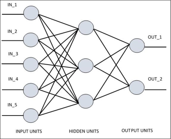
Fig. 1  Deep Learning using ANN - System Architecture

The diagram shows that the hidden units communicate with the external layer. While the input and output units communicate only through the hidden layer of the network.

The pattern of connection with nodes, the total number of layers and level of nodes between inputs and outputs with the number of neurons per layer define the architecture of a neural network.

There are two types of architecture. These types focus on the functionality artificial neural networks as follows −

1. Single Layer Perceptron
2. Multi-Layer Perceptron

Single Layer Perceptron

Single layer perceptron is the first proposed neural model created. The content of the local memory of the neuron consists of a vector of weights. The computation of a single layer perceptron is performed over the calculation of sum of the input vector each with the value multiplied by corresponding element of vector of the weights. The value which is displayed in the output will be the input of an activation function.

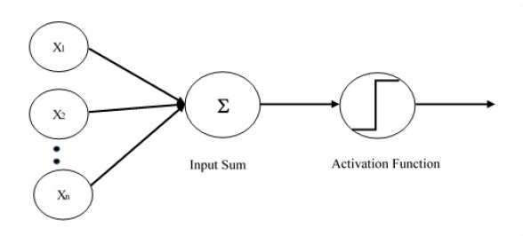
Fig. 2 Single Layer Perceptron (SLP) - System Architecture

Let us focus on the implementation of single layer perceptron for an image classification problem using TensorFlow. The best example to illustrate the single layer perceptron is through representation of “Logistic Regression”.

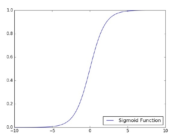
Fig. 3 Activation Function using Sigmoid Function

Now, let us consider the following basic steps of training logistic regression −

- The weights are initialized with random values at the beginning of the training.

- For each element of the training set, the error is calculated with the difference between desired output and the actual output. The error calculated is used to adjust the weights.

- The process is repeated until the error made on the entire training set is not less than the specified threshold, until the maximum number of iterations is reached.

TensorFlow

TensorFlow is an open source software library created by Google for numerical computation using data flow graphs.

Nodes in the graph represent mathematical operations, while the graph edges represent the multidimensional data arrays (tensors) that flow between them. This flexible architecture lets you deploy computation to one or more CPU's or GPU’s in a desktop, server, or mobile device without rewriting code.

TensorFlow also includes TensorBoard, a data visualization toolkit.

Building a SLP in TensorFlow

Dataset

In this article, we will be using MNIST, a data-set of handwritten digits (The “hello world” of image recognition for machine learning and deep learning).

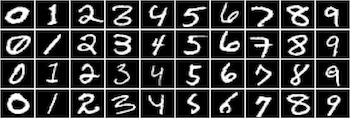
Fig. 4 MNIST Sample Images

It is a digit recognition task. There are 10 digits (0 to 9) or 10 classes to predict. Each image is a 28 by 28 pixel square (784 pixels total). We’re given a total of 70,000 images.

Python Code of SLP using TensorFlow

Step 1 - Launch Python TensorFlow (eg.) from Anaconda Spyder

Step 2 - Import Packages

import tensorflow as tf import numpy as np import matplotlib.pyplot as plt %matplotlib inline import time

Step 3 - Load MNIST Data

# Import MNIST data from tensorflow.examples.tutorials.mnist import input_data mnist = input_data.read_data_sets("/tmp/data/", one_hot=True)

You should see something like this:

Extracting data/MNIST/train-images-idx3-ubyte.gz
Extracting data/MNIST/train-labels-idx1-ubyte.gz
Extracting data/MNIST/t10k-images-idx3-ubyte.gz
Extracting data/MNIST/t10k-labels-idx1-ubyte.gz

Check the data by typing:

print("Size of:") print("- Training-set:\t\t{}".format(len(data.train.labels))) print("- Test-set:\t\t{}".format(len(data.test.labels))) print("- Validation-set:\t{}".format(len(data.validation.labels)))

You should see something like this:

Size of:
- Training-set: 55000
- Test-set: 10000
- Validation-set: 5000

Step 4 - Set MLP Parameters# Parameters

learning_rate = 0.01 training_epochs = 50 batch_size = 100 display_step = 1

Step 5 - Set x & y Placeholders

# tf Graph Input x = tf.placeholder("float", [None, 784]) # mnist data image of shape 28*28 = 784 y = tf.placeholder("float", [None, 10]) # 0-9 digits recognition => 10 classes

Step 6 - Define weights and bias

# Create model # Set model weights W = tf.Variable(tf.zeros([784, 10])) b = tf.Variable(tf.zeros([10]))

Step 7 - Construct Model

# Construct model activation = tf.nn.softmax(tf.matmul(x, W) + b) # Softmax

Step 8 - Define Cross Entropy too minimize error

# Minimize error using cross entropy cross_entropy = y*tf.log(activation) cost = tf.reduce_mean(-tf.reduce_sum (cross_entropy,reduction_indices = 1)) optimizer = tf.train.GradientDescentOptimizer(learning_rate).minimize(cost)

Step 9 - Define plot settings (Average cost vs. Epochs)

#Plot settings avg_set = [] epoch_set = []

Step 10 - Initial Variables

# Initializing the variables init = tf.initialize_all_variables()

Step 11 - Launch SLP Sessions

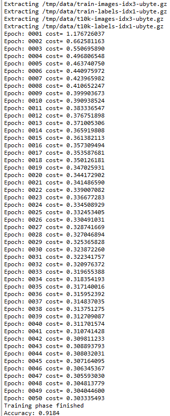
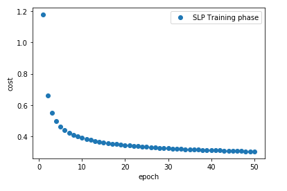
# Launch the graph with tf.Session() as sess: sess.run(init) # Training cycle for epoch in range(training_epochs): avg_cost = 0. total_batch = int(mnist.train.num_examples/batch_size) # Loop over all batches for i in range(total_batch): batch_xs, batch_ys = mnist.train.next_batch(batch_size) # Fit training using batch data sess.run(optimizer, feed_dict = {x: batch_xs, y: batch_ys}) # Compute average loss avg_cost += sess.run(cost, feed_dict = {x: batch_xs, y: batch_ys})/total_batch # Display logs per epoch step if epoch % display_step == 0: print("Epoch:", '%04d' % (epoch+1), "cost=", "{:.9f}".format(avg_cost)) avg_set.append(avg_cost) epoch_set.append(epoch+1) print("Training phase finished") # Test model correct_prediction = tf.equal(tf.argmax(activation, 1), tf.argmax(y, 1)) # Calculate accuracy accuracy = tf.reduce_mean(tf.cast(correct_prediction, "float")) print("Accuracy:", accuracy.eval({x: mnist.test.images, y: mnist.test.labels})) plt.plot(epoch_set,avg_set, 'o', label = 'SLP Training phase') plt.ylabel('cost') plt.xlabel('epoch') plt.legend() plt.show()

The above line of code generates the following output −

Execute your SLP TensorFlow program to see whether you can got similar results:

The Performance Chart should look like this.

The logistic regression is considered as a predictive analysis. Logistic regression is used to describe data and to explain the relationship between one dependent binary variable and one or more nominal or independent variables.

Next, we will implement Multi-Layer Perceptron (MLP) using TensorFlow and see how it works.