Convolutional Neural Networks

Originally developed by Yann LeCun decades ago, better known as CNNs (ConvNets) are one of the state of the art, Artificial Neural Network design architecture, which has proven its effectiveness in areas such as image recognition and classification. The Basic Principle behind the working of CNN is the idea of Convolution, producing filtered Feature Maps stacked over each other.

A convolutional neural network consists of several layers. Implicit explanation about each of these layers is given below.

1. Convolution Layer (Conv Layer)

The Conv layer is the core building block of a Convolutional Neural Network. The primary purpose of Conv layer is to extract features from the input image.

Fig 1 Convolution Mechanism

The Conv Layer parameters consist of a set of learnable filters (kernels or feature detector). Filters are used for recognizing patterns throughout the entire input image. Convolution works by sliding the filter over the input image and along the way we take the dot product between the filter and chunks of the input image.

2. Pooling Layer (Sub-sampling or Down-sampling)

Pooling layer reduce the size of feature maps by using some functions to summarize sub-regions, such as taking the average or the maximum value. Pooling works by sliding a window across the input and feeding the content of the window to a pooling function.

Fig.2 Max-Pooling and Average-Pooling

The purpose of pooling is to reduce the number of parameters in our network (hence called down-sampling) and to make learned features more robust by making it more invariant to scale and orientation changes.

3. ReLU Layer

ReLU stands for Rectified Linear Unit and is a non-linear operation. ReLU is an element wise operation (applied per pixel) and replaces all negative pixel values in the feature map by zero.

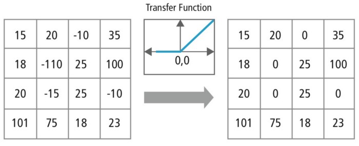
Fig. 3 ReLU Layer

The purpose of ReLU is to introduce non-linearity in our ConvNet, since most of the real-world data we would want our ConvNet to learn would be non-linear.

Other non linear functions such as tanh or sigmoid can also be used instead of ReLU, but ReLU has been found to perform better in most cases.

4. Fully Connected Layer

The Fully Connected layer is configured exactly the way its name implies: it is fully connected with the output of the previous layer. A fully connected layer takes all neurons in the previous layer (be it fully connected, pooling, or convolutional) and connects it to every single neuron it has.

Fig. 4 Fully Connected Layer

Adding a fully-connected layer is also a cheap way of learning non-linear combinations of these features. Most of the features learned from convolutional and pooling layers may be good, but combinations of those features might be even better.

TensorFlow

TensorFlow is an open source software library created by Google for numerical computation using data flow graphs.

Nodes in the graph represent mathematical operations, while the graph edges represent the multidimensional data arrays (tensors) that flow between them. This flexible architecture lets you deploy computation to one or more CPU's or GPU’s in a desktop, server, or mobile device without rewriting code.

TensorFlow also includes TensorBoard, a data visualization toolkit.

Building a CNN in TensorFlow

Dataset

In this article, we will be using MNIST, a data-set of handwritten digits (The “hello world” of image recognition for machine learning and deep learning).

Fig. 5 MNIST Sample Images

It is a digit recognition task. There are 10 digits (0 to 9) or 10 classes to predict. Each image is a 28 by 28 pixel square (784 pixels total). We’re given a total of 70,000 images.

Network Architecture

• Convolution, Filter shape:(5,5,6), Stride=1, Padding=’SAME’
• Max pooling (2x2), Window shape:(2,2), Stride=2, Padding=’Same’
• ReLU
• Convolution, Filter shape:(5,5,16), Stride=1, Padding=’SAME’
• Max pooling (2x2), Window shape:(2,2), Stride=2, Padding=’Same’
• ReLU
• Fully Connected Layer (128)
• ReLU
• Fully Connected Layer (10)
• Softmax

Fig.7 CNN System Architecture

Python Code

Step 1 - Launch Python TensorFlow (eg.) from Anaconda Spyder

Step 2 - Import Packages

import tensorflow as tf import numpy as np import matplotlib.pyplot as plt %matplotlib inline import time

Step 3 - Load Data

from tensorflow.examples.tutorials.mnist import input_data data = input_data.read_data_sets('data/MNIST/', one_hot=True)

You should see something like this:

Extracting data/MNIST/train-images-idx3-ubyte.gz
Extracting data/MNIST/train-labels-idx1-ubyte.gz
Extracting data/MNIST/t10k-images-idx3-ubyte.gz
Extracting data/MNIST/t10k-labels-idx1-ubyte.gz

Check the data by typing:

print("Size of:") print("- Training-set:\t\t{}".format(len(data.train.labels))) print("- Test-set:\t\t{}".format(len(data.test.labels))) print("- Validation-set:\t{}".format(len(data.validation.labels)))

You should see something like this:

Size of:
- Training-set: 55000
- Test-set: 10000
- Validation-set: 5000

Step 4 - Placeholder variables

# Placeholder variable for the input images x = tf.placeholder(tf.float32, shape=[None, 28*28], name='X') # Reshape it into [num_images, img_height, img_width, num_channels] x_image = tf.reshape(x, [-1, 28, 28, 1]) # Placeholder variable for the true labels associated with the images y_true = tf.placeholder(tf.float32, shape=[None, 10], name='y_true') y_true_cls = tf.argmax(y_true, dimension=1)

Step 5 - Function for creating a new Convolution Layer

def new_conv_layer(input, num_input_channels, filter_size, num_filters, name): with tf.variable_scope(name) as scope: # Shape of the filter-weights for the convolution shape = [filter_size, filter_size, num_input_channels, num_filters] # Create new weights (filters) with the given shape weights = tf.Variable(tf.truncated_normal(shape, stddev=0.05)) # Create new biases, one for each filter biases = tf.Variable(tf.constant(0.05, shape=[num_filters])) # TensorFlow operation for convolution layer = tf.nn.conv2d(input=input, filter=weights, strides=[1, 1, 1, 1], padding='SAME') # Add the biases to the results of the convolution. layer += biases return layer, weights

Step 6 - Function for creating a new Pooling Layer

def new_pool_layer(input, name): with tf.variable_scope(name) as scope: # TensorFlow operation for convolution layer = tf.nn.max_pool(value=input, ksize=[1, 2, 2, 1], strides=[1, 2, 2, 1], padding='SAME') return layer

Step 7 - Function for creating a new ReLU Layer

def new_relu_layer(input, name): with tf.variable_scope(name) as scope: # TensorFlow operation for convolution layer = tf.nn.relu(input) return layer

Step 8 - Function for creating a new Fully connected Layer

def new_fc_layer(input, num_inputs, num_outputs, name): with tf.variable_scope(name) as scope: # Create new weights and biases. weights = tf.Variable(tf.truncated_normal([num_inputs, num_outputs], stddev=0.05)) biases = tf.Variable(tf.constant(0.05, shape=[num_outputs])) # Multiply the input and weights, and then add the bias-values. layer = tf.matmul(input, weights) + biases return layer

Step 9 - Create Convolutional Neural Network

# Convolutional Layer 1 layer_conv1, weights_conv1 = new_conv_layer(input=x_image, num_input_channels=1, filter_size=5, num_filters=6, name ="conv1") # Pooling Layer 1 layer_pool1 = new_pool_layer(layer_conv1, name="pool1") # RelU layer 1 layer_relu1 = new_relu_layer(layer_pool1, name="relu1") # Convolutional Layer 2 layer_conv2, weights_conv2 = new_conv_layer(input=layer_relu1, num_input_channels=6, filter_size=5, num_filters=16, name= "conv2") # Pooling Layer 2 layer_pool2 = new_pool_layer(layer_conv2, name="pool2") # RelU layer 2 layer_relu2 = new_relu_layer(layer_pool2, name="relu2") # Flatten Layer num_features = layer_relu2.get_shape()[1:4].num_elements() layer_flat = tf.reshape(layer_relu2, [-1, num_features]) # Fully-Connected Layer 1 layer_fc1 = new_fc_layer(layer_flat, num_inputs=num_features, num_outputs=128, name="fc1") # RelU layer 3 layer_relu3 = new_relu_layer(layer_fc1, name="relu3") # Fully-Connected Layer 2 layer_fc2 = new_fc_layer(input=layer_relu3, num_inputs=128, num_outputs=10, name="fc2")

Step 10 - Softmax function to normalize the output

# Use Softmax function to normalize the output with tf.variable_scope("Softmax"): y_pred = tf.nn.softmax(layer_fc2) y_pred_cls = tf.argmax(y_pred, dimension=1)

Step 11 - Cost Function

# Use Cross entropy cost function with tf.name_scope("cross_ent"): cross_entropy = tf.nn.softmax_cross_entropy_with_logits(logits=layer_fc2, labels=y_true) cost = tf.reduce_mean(cross_entropy)

Step 12 - Optimizer

# Use Adam Optimizer with tf.name_scope("optimizer"): optimizer = tf.train.AdamOptimizer(learning_rate=1e-4).minimize(cost)

Step 13 - Accuracy

# Accuracy with tf.name_scope("accuracy"): correct_prediction = tf.equal(y_pred_cls, y_true_cls) accuracy = tf.reduce_mean(tf.cast(correct_prediction, tf.float32))

Step 14 - FileWriter

# Initialize the FileWriter writer = tf.summary.FileWriter("Training_FileWriter/") writer1 = tf.summary.FileWriter("Validation_FileWriter/")

Step 15 - Set Summary data

# Add the cost and accuracy to summary tf.summary.scalar('loss', cost) tf.summary.scalar('accuracy', accuracy) # Merge all summaries together merged_summary = tf.summary.merge_all()

Step 16 - Set Epoch and batch size parameters

num_epochs = 100 batch_size = 100

Step 16 - TensorFlow Session

with tf.Session() as sess: # Initialize all variables sess.run(tf.global_variables_initializer()) # Add the model graph to TensorBoard writer.add_graph(sess.graph) # Loop over number of epochs for epoch in range(num_epochs): start_time = time.time() train_accuracy = 0 for batch in range(0, int(len(data.train.labels)/batch_size)): # Get a batch of images and labels x_batch, y_true_batch = data.train.next_batch(batch_size) # Put the batch into a dict with the proper names for placeholder variables feed_dict_train = {x: x_batch, y_true: y_true_batch} # Run the optimizer using this batch of training data. sess.run(optimizer, feed_dict=feed_dict_train) # Calculate the accuracy on the batch of training data train_accuracy += sess.run(accuracy, feed_dict=feed_dict_train) # Generate summary with the current batch of data and write to file summ = sess.run(merged_summary, feed_dict=feed_dict_train) writer.add_summary(summ, epoch*int(len(data.train.labels)/batch_size) + batch) train_accuracy /= int(len(data.train.labels)/batch_size) # Generate summary and validate the model on the entire validation set summ, vali_accuracy = sess.run([merged_summary, accuracy], feed_dict={x:data.validation.images, y_true:data.validation.labels}) writer1.add_summary(summ, epoch) end_time = time.time() print("Epoch "+str(epoch+1)+" completed : Time usage "+str(int(end_time-start_time))+" seconds") print("\tAccuracy:") print ("\t- Training Accuracy:\t{}".format(train_accuracy)) print ("\t- Validation Accuracy:\t{}".format(vali_accuracy))

Training Results (First 50 Epochs)
- Try the TensorFlow CNN program, see whether you have better results.

Epoch 1 completed : Time usage 106 seconds Accuracy: - Training Accuracy: 0.7252181817354126 - Validation Accuracy: 0.9010000228881836 Epoch 2 completed : Time usage 101 seconds Accuracy: - Training Accuracy: 0.9172909103740345 - Validation Accuracy: 0.9350000023841858 Epoch 3 completed : Time usage 97 seconds Accuracy: - Training Accuracy: 0.9371818196773529 - Validation Accuracy: 0.9484000205993652 Epoch 4 completed : Time usage 101 seconds Accuracy: - Training Accuracy: 0.9475090927427465 - Validation Accuracy: 0.9588000178337097 Epoch 5 completed : Time usage 92 seconds Accuracy: - Training Accuracy: 0.9547454566305333 - Validation Accuracy: 0.9607999920845032 Epoch 6 completed : Time usage 93 seconds Accuracy: - Training Accuracy: 0.959872730103406 - Validation Accuracy: 0.9679999947547913 Epoch 7 completed : Time usage 98 seconds Accuracy: - Training Accuracy: 0.9643272785706953 - Validation Accuracy: 0.968999981880188 Epoch 8 completed : Time usage 105 seconds Accuracy: - Training Accuracy: 0.9679454628987746 - Validation Accuracy: 0.9728000164031982 Epoch 9 completed : Time usage 98 seconds Accuracy: - Training Accuracy: 0.9708000080151992 - Validation Accuracy: 0.9764000177383423 Epoch 10 completed : Time usage 99 seconds Accuracy: - Training Accuracy: 0.9735091001337225 - Validation Accuracy: 0.9765999913215637 Epoch 11 completed : Time usage 97 seconds Accuracy: - Training Accuracy: 0.9753454634276303 - Validation Accuracy: 0.9783999919891357 Epoch 12 completed : Time usage 103 seconds Accuracy: - Training Accuracy: 0.9768909192085267 - Validation Accuracy: 0.9800000190734863 Epoch 13 completed : Time usage 99 seconds Accuracy: - Training Accuracy: 0.9785818283124403 - Validation Accuracy: 0.9789999723434448 Epoch 14 completed : Time usage 95 seconds Accuracy: - Training Accuracy: 0.9796000105684454 - Validation Accuracy: 0.9815999865531921 Epoch 15 completed : Time usage 96 seconds Accuracy: - Training Accuracy: 0.9813272833824158 - Validation Accuracy: 0.9810000061988831 Epoch 16 completed : Time usage 103 seconds Accuracy: - Training Accuracy: 0.982036375132474 - Validation Accuracy: 0.9843999743461609 Epoch 17 completed : Time usage 97 seconds Accuracy: - Training Accuracy: 0.982872737754475 - Validation Accuracy: 0.9850000143051147 Epoch 18 completed : Time usage 97 seconds Accuracy: - Training Accuracy: 0.9842363735762509 - Validation Accuracy: 0.984000027179718 Epoch 19 completed : Time usage 97 seconds Accuracy: - Training Accuracy: 0.9848363750631159 - Validation Accuracy: 0.9842000007629395 Epoch 20 completed : Time usage 97 seconds Accuracy: - Training Accuracy: 0.985927283222025 - Validation Accuracy: 0.9851999878883362 Epoch 21 completed : Time usage 95 seconds Accuracy: - Training Accuracy: 0.9864727374640379 - Validation Accuracy: 0.9868000149726868 Epoch 22 completed : Time usage 101 seconds Accuracy: - Training Accuracy: 0.9869454645026814 - Validation Accuracy: 0.9861999750137329 Epoch 23 completed : Time usage 100 seconds Accuracy: - Training Accuracy: 0.9873272825371135 - Validation Accuracy: 0.9873999953269958 Epoch 24 completed : Time usage 101 seconds Accuracy: - Training Accuracy: 0.9876727361028844 - Validation Accuracy: 0.9876000285148621 Epoch 25 completed : Time usage 97 seconds Accuracy: - Training Accuracy: 0.9885454641688953 - Validation Accuracy: 0.9873999953269958 Epoch 26 completed : Time usage 97 seconds Accuracy: - Training Accuracy: 0.9887818276882172 - Validation Accuracy: 0.9869999885559082 Epoch 27 completed : Time usage 98 seconds Accuracy: - Training Accuracy: 0.9892181905833157 - Validation Accuracy: 0.9864000082015991 Epoch 28 completed : Time usage 101 seconds Accuracy: - Training Accuracy: 0.9898909175395966 - Validation Accuracy: 0.9886000156402588 Epoch 29 completed : Time usage 109 seconds Accuracy: - Training Accuracy: 0.9899454631588676 - Validation Accuracy: 0.9887999892234802 Epoch 30 completed : Time usage 101 seconds Accuracy: - Training Accuracy: 0.9904909170757641 - Validation Accuracy: 0.9865999817848206 Epoch 31 completed : Time usage 112 seconds Accuracy: - Training Accuracy: 0.991036371534521 - Validation Accuracy: 0.9882000088691711 Epoch 32 completed : Time usage 105 seconds Accuracy: - Training Accuracy: 0.9911454620144584 - Validation Accuracy: 0.9896000027656555 Epoch 33 completed : Time usage 103 seconds Accuracy: - Training Accuracy: 0.9916545529799028 - Validation Accuracy: 0.9887999892234802 Epoch 34 completed : Time usage 95 seconds Accuracy: - Training Accuracy: 0.9922545524076982 - Validation Accuracy: 0.9883999824523926 Epoch 35 completed : Time usage 93 seconds Accuracy: - Training Accuracy: 0.9919454616850073 - Validation Accuracy: 0.9886000156402588 Epoch 36 completed : Time usage 92 seconds Accuracy: - Training Accuracy: 0.9927272792295976 - Validation Accuracy: 0.9894000291824341 Epoch 37 completed : Time usage 94 seconds Accuracy: - Training Accuracy: 0.993454551154917 - Validation Accuracy: 0.9891999959945679 Epoch 38 completed : Time usage 94 seconds Accuracy: - Training Accuracy: 0.9932545514540239 - Validation Accuracy: 0.9894000291824341 Epoch 39 completed : Time usage 93 seconds Accuracy: - Training Accuracy: 0.9930727336623452 - Validation Accuracy: 0.989799976348877 Epoch 40 completed : Time usage 93 seconds Accuracy: - Training Accuracy: 0.9941090965270996 - Validation Accuracy: 0.989799976348877 Epoch 41 completed : Time usage 92 seconds Accuracy: - Training Accuracy: 0.9937090969085693 - Validation Accuracy: 0.9901999831199646 Epoch 42 completed : Time usage 93 seconds Accuracy: - Training Accuracy: 0.994454550634731 - Validation Accuracy: 0.9894000291824341 Epoch 43 completed : Time usage 93 seconds Accuracy: - Training Accuracy: 0.9946000050414693 - Validation Accuracy: 0.9908000230789185 Epoch 44 completed : Time usage 95 seconds Accuracy: - Training Accuracy: 0.9951272773742675 - Validation Accuracy: 0.9894000291824341 Epoch 45 completed : Time usage 93 seconds Accuracy: - Training Accuracy: 0.9949090957641602 - Validation Accuracy: 0.9911999702453613 Epoch 46 completed : Time usage 92 seconds Accuracy: - Training Accuracy: 0.9951454589583657 - Validation Accuracy: 0.9896000027656555 Epoch 47 completed : Time usage 93 seconds Accuracy: - Training Accuracy: 0.9953818225860596 - Validation Accuracy: 0.9909999966621399 Epoch 48 completed : Time usage 93 seconds Accuracy: - Training Accuracy: 0.9955272769927979 - Validation Accuracy: 0.9904000163078308 Epoch 49 completed : Time usage 93 seconds Accuracy: - Training Accuracy: 0.9957818220962178 - Validation Accuracy: 0.9904000163078308 Epoch 50 completed : Time usage 93 seconds Accuracy: - Training Accuracy: 0.9957090950012207 - Validation Accuracy: 0.9904000163078308 ...

We can plot the validation accuracy and loss versus the number of epoch’s using TensorBoard :

Step 1: After finish the 100 epochs, launch Anaconda DOS prompt

Step 2: Goto your Lab drive and directory

Step 3: Using "dir" to check whether directory "Validation_FileWriter" exist.

Step 4: Launch TensorBoard by typing "tensorboard --logdir Validation_FileWriter"

Step 5: In your browser, type "http://localhost:6006" to open Tensorboard.

You should see this:

Step 6: You can click the "CSV" links to download all the data (accuracy and loss) into CSV files.

With minimal efforts, we managed to reach an accuracy of 99% which is not that bad for a classification task with 10 labels.

This result has been achieved without extensive optimization of the convolutional neural network’s parameters, and also without any form of regularization.

To improve the performances, we could set up more complex model architectures so as to refine the feature extraction.

See the results of our Convolutional Neural Network on some validation examples:

Fig.10 MNIST Sample Classifications

Conclusion

In this lab, we were able to implement the simple Convolutional Neural Network architecture using the Python programming language and the TensorFlow library for deep learning.